Monitor one reading at a time

Monitor one reading at a time

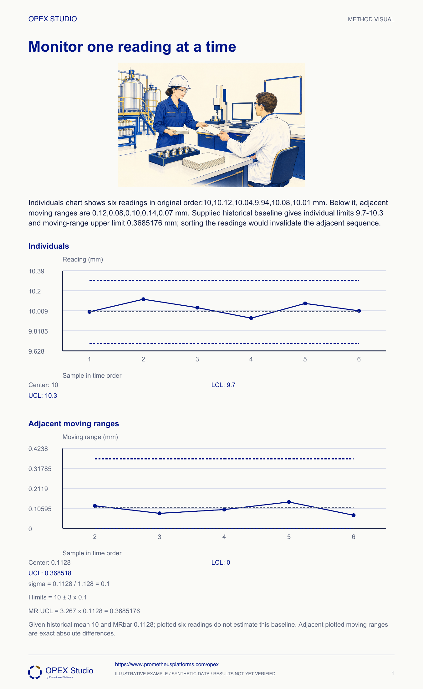
When only one measurement is available at each observation time, an individuals chart may be appropriate. The moving range uses the absolute difference between adjacent readings in their original order. Sorting values before taking differences destroys the time structure and understates what the process experienced. In this example the historical moving-range average estimates a short-term standard deviation using the stated constant. The short plotted sequence is illustrative and is not used to estimate that baseline. Check dependence, measurement fitness and process context before adopting the method. A signal should trigger the defined investigation; it is not automatically a command to adjust equipment.

Follow the method

1. Individuals
2. Reading (mm)
3. Sample in time order
4. Center: 10
5. LCL: 9.7
6. UCL: 10.3
7. Adjacent moving ranges
8. Moving range (mm)
9. Center: 0.1128
10. LCL: 0
11. UCL: 0.368518

Separate historical limits from later observations

Fictional case: Juniper Batch records one width per batch. Supplied historical mean is 10.00 mm and MRbar is 0.1128 mm. Six subsequent illustrative readings are 10.00,10.12,10.04,9.94,10.08,10.01 mm. Analyst Owen checks the individuals and moving-range records. The core exhibit retains these exact values and historical parameters.

Follow the method

1. Sigma from historical MRbar
2. Individuals limits
3. MR limits
4. Later illustration

The gap between neighbors matters

Calculate adjacent moving ranges and use supplied historical limits without losing time order or turning a signal into an equipment command.

Fictional case: Juniper Batch records one width per batch. Supplied historical mean is 10.00 mm and MRbar is 0.1128 mm. Six subsequent illustrative readings are 10.00,10.12,10.04,9.94,10.08,10.01 mm. Analyst Owen checks the individuals and moving-range records. The core exhibit retains these exact values and historical parameters.

Role: Process analyst and batch-record owner

Normal condition

Each reading retains its batch order and measurement context; moving ranges compare successive observations; baseline assumptions and the reaction rule are explicit.

The gap

A spreadsheet sorts readings before calculating ranges and derives a new baseline from the six-point illustration.

• A single measurement per batch does not guarantee independence.
• This calculation lesson does not establish a process capability study or prescribe a machine adjustment.

1. Protect observation order

   Owen preserves batch identity and timestamps before calculating differences. The first plotted reading has no within-sequence previous observation, so this six-point sequence has five moving ranges.

   Why: Sorting changes neighbors and therefore changes the statistic. A visually smoother range chart made from sorted values would no longer describe batch-to-batch behavior.

   Evidence: Six ordered readings and five correctly aligned moving ranges.

2. Recalculate the adjacent differences

   He takes absolute differences:|10.12−10.00|=.12, then .08,.10,.14,.07 mm. Each moving range belongs to the later member of its pair.

   Why: Absolute differences measure the size of the neighboring change; their sign is not plotted as spread. Keeping alignment helps trace a signal to both involved observations.

   Evidence: The raw pair for every range is recoverable.

3. Use the supplied historical estimate

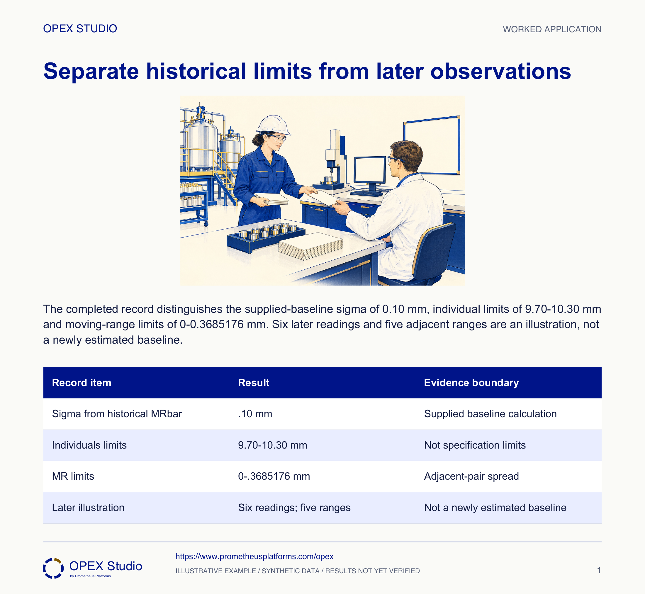
   Historical sigma estimate is .1128/1.128=.10 mm. Individuals limits are 10 ±3×.10, giving 9.70 and 10.30 mm. The MR upper limit is 3.267×.1128=.3685176 mm, with lower limit 0.

   Why: The historical MRbar is an explicit input. The average of the five displayed ranges is .102 mm, which is not substituted for that baseline.

   Evidence: Calculation record distinguishes historical parameters from later demonstration points.

4. Interpret the displayed sequence narrowly

   The six readings and five ranges have no beyond-limit point under the stated point rule. Owen checks dependence and operating context before making broader statements.

   Why: Smooth autocorrelated data can yield misleading short-range estimates. Six quiet points do not demonstrate that all assumptions are adequate or that future behavior is stable.

   Evidence: The report states the checked rule and the limits of the illustration.

5. Prepare a traceable reaction

   For any signal he records the batch pair, measurement condition, known changes and authorized response. He does not convert a positive error or large range into a knob-turning instruction.

   Why: A chart detects evidence worth investigating; the process authority determines safe containment, correction and restart. Preserving the original result supports learning about causes.

   Evidence: The response record contains observations and roles, with no invented operating command.

A new reading jumps to 10.50 mm

After the last illustrative reading 10.01 mm, the next fictional observation is 10.50 mm.

Record both the individuals signal 10.50>10.30 and moving range .49>.3685176. Retain both batch identities and follow the approved abnormality response.

The moving range links the jump to its neighbor; it does not identify which physical cause produced it.

Two signals are recorded against the same unchanged baseline.

Run a practice session

Materials

• Ordered batch cards
• Calculator
• Blank pair-to-range table

1. Identify neighbors · 5 minutes

   Why are there five ranges for six displayed readings?

2. Compare historical and plotted averages · 8 minutes

   Which baseline is this exercise using?

3. Complete the 5 mm sequence · 10 minutes

   Which records belong in the investigation?

4. Debrief · 5 minutes

   How would dependence affect confidence in the method?

Debrief

• Ask learners to calculate one range aloud from its two readings.
• Do not let a correct limit calculation imply adequate sampling design.

Preserve the written observation order and annotate each difference between adjacent rows.

Transfer into the work

Owner: SPC analyst and batch-process owner

Record: Ordered measurements, baseline revision and pair-linked response log

Review: At each defined observation and during baseline review

Evidence: Correct pair alignment, measurement fitness and verified response

Investigate dependence or process changes; do not conceal signals through sorting or automatic rebaselining.