Facilitator guide
Case objectives, demonstration plans, debriefs, common mistakes and application checks across all 81 workplace cases and method lessons.
Download Facilitator guide PDF · 166 pages · 65.1 MB OPEXSTUDIO
Separate measurements, nonconforming units and nonconformities.. Follow the visual, practise a decision, then check your thinking.
Fictional teaching examples and AI-generated illustrations. Proposed changes and goals are not achieved results. Use the written instructions and check local conditions before applying a method.
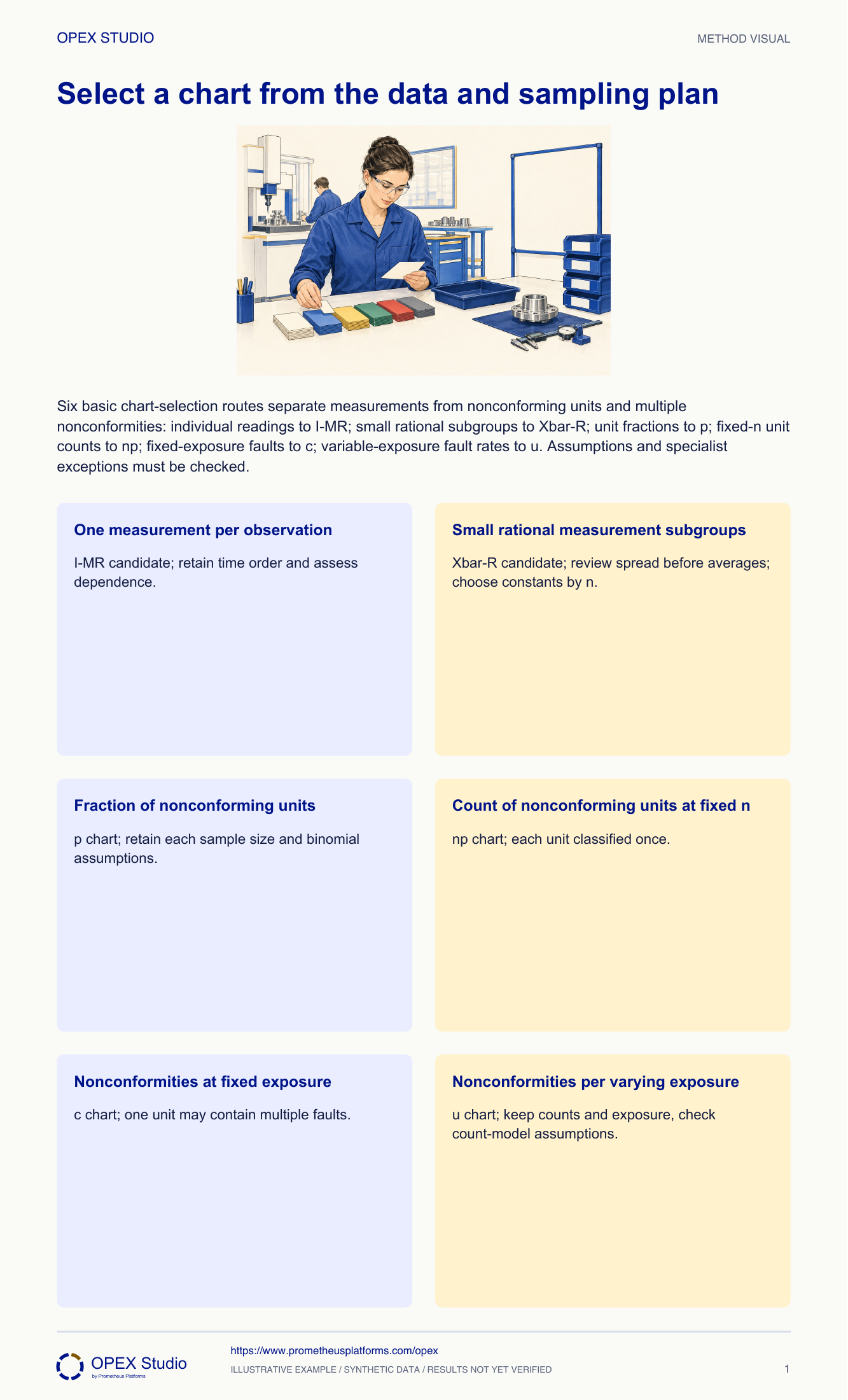
Chart selection starts with how data are generated. Measurements taken individually differ from rational subgroups collected under comparable short-term conditions. Nonconforming units differ from nonconformities, because one unit can contain several faults. For attributes, record whether the inspected quantity or exposure changes. These distinctions guide the candidate family: individuals and moving range, subgroup charts, p or np, and c or u. Selection is not complete until independence and model assumptions are considered. Rare events, autocorrelation, changing opportunity and overdispersion may require specialist methods. Choose the sampling plan and interpretation rules before routine monitoring begins.
Measurements differ from counts; units differ from nonconformities.
p/np classify units once; c/u can count several faults per unit.
Independence, subgroup rationale and exposure must be checked.
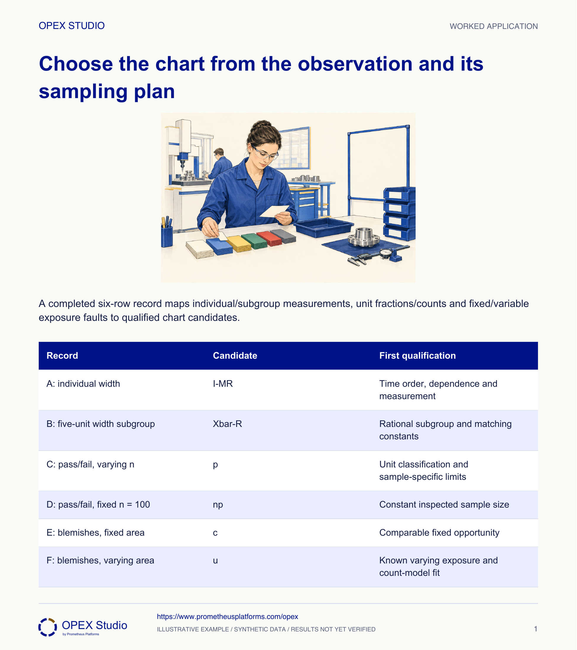
Fictional case: a monitoring workshop receives six records: individual widths, small width subgroups, rejected-unit fractions, fixed-size reject counts, fixed-area blemish counts and varying-area blemish rates. The core chooser retains six distinct routes. Engineer Sal must assign candidates without pretending that a chart name approves the collection plan.
Retrieve the actual denominators before calculating fractions or limits. Mark the missing observations explicitly; do not assume 100 because another row uses 100.
A plausible-looking graph based on invented exposure would communicate false evidence. Another process’s denominator is not a substitute.
Select a monitoring candidate from the observation type and sampling design, then identify the assumptions that still need review.
Fictional case: a monitoring workshop receives six records: individual widths, small width subgroups, rejected-unit fractions, fixed-size reject counts, fixed-area blemish counts and varying-area blemish rates. The core chooser retains six distinct routes. Engineer Sal must assign candidates without pretending that a chart name approves the collection plan.
Role: Quality engineer and process record owner
The team knows what one observation means, its time order, subgroup or exposure basis and whether a unit can contribute more than one event.
Every record has been labelled defects. A proposed p chart would treat multiple blemishes on one sheet as though they were different rejected sheets.
| Record | Collection design |
|---|---|
| A: width | One measurement per time point |
| B: width | Five consecutive units per subgroup |
| C: pass/fail units | Known sample sizes that vary |
| D: pass/fail units | Always 100 inspected per sample |
| E: blemishes | Same inspected area each time |
| F: blemishes | Different known areas each time |
Sal marks A and B as measured variables. C and D classify each unit once. E and F can record several nonconformities within one inspection area.
Why: The number format alone is insufficient: both widths and defect counts are numbers. The observation definition determines the statistical question.
Evidence: Each record names its unit and whether multiple events can belong to it.
For A he retains time order and considers I–MR. For B he examines whether five consecutive units are a rational subgroup under comparable conditions and considers Xbar–R.
Why: A subgroup is an intentional comparison structure, not any five values pooled for convenience. Serial dependence and measurement fitness can invalidate a simple chart choice.
Evidence: Candidate A is I–MR; B is Xbar–R subject to subgroup and measurement review.
C uses a p candidate because each sample has a known denominator that may change. D can use an np candidate for the count because its denominator remains 100.
Why: A raw count rises when more units are inspected even if the fraction is unchanged. Fixed-n and variable-n displays must retain their intended scale.
Evidence: The selection record preserves each sample size and binomial-model questions.
E uses a c candidate only with comparable fixed exposure. F uses a u candidate with count divided by known exposure and exposure-dependent limits.
Why: Counting blemishes is not the same as classifying a sheet once. A larger area provides more opportunity, and count-model assumptions need scrutiny.
Evidence: The record defines the exposure unit and distinguishes multiple faults from affected items.
Sal records unresolved dependence, opportunity, measurement and response-plan questions. A chart owner must confirm baseline development and reaction rules before operational use.
Why: Choosing a plausible chart is a first decision. It does not establish stability, approve product release or authorize automatic adjustments.
Evidence: Every row has a candidate and at least one explicit qualification check.
| Record | Candidate | First qualification |
|---|---|---|
| A: individual width | I–MR | Time order, dependence and measurement |
| B: five-unit width subgroup | Xbar–R | Rational subgroup and matching constants |
| C: pass/fail, varying n | p | Unit classification and sample-specific limits |
| D: pass/fail, fixed n = 100 | np | Constant inspected sample size |
| E: blemishes, fixed area | c | Comparable fixed opportunity |
| F: blemishes, varying area | u | Known varying exposure and count-model fit |
Record C gives rejected units but omits how many were inspected on two days.
Retrieve the actual denominators before calculating fractions or limits. Mark the missing observations explicitly; do not assume 100 because another row uses 100.
A plausible-looking graph based on invented exposure would communicate false evidence. Another process’s denominator is not a substitute.
The record identifies the two missing sample sizes and their owner.
New fictional records contain one service duration per completed case, six measurements collected across different machines, multiple faults over varying inspected cable lengths, and pass/fail counts from a fixed 50-unit sample.
| Record | Design issue |
|---|---|
| Service duration | One observation at each completion |
| Six measurements | Mixed machines in one proposed subgroup |
| Cable faults | Known varying length |
| Pass/fail | Fixed n=50 |
I–MR is a candidate for individual duration, subject to distribution/dependence and measurement review. The six mixed-machine readings are not automatically a rational subgroup; preserve source identity and design the grouping first.
Use u as a candidate for multiple faults per varying cable length, and np for nonconforming-unit count at fixed 50. A p display of the same fixed-size unit fractions is also defensible if its scale is clear.
| Record | Candidate or action | Boundary |
|---|---|---|
| Duration | I–MR candidate | Assess dependence and distribution |
| Mixed measurements | Repair subgroup design | Do not pool unlike conditions casually |
| Cable faults | u candidate | Known comparable opportunity per length |
| Fixed 50 pass/fail | np or clearly labelled p | One classification per unit |
Can one item contribute more than one count?
What changes when n or exposure changes?
What variation would pooling hide?
Who approves the baseline and response?
Annotate the sampling mechanism before looking up any chart name.
Owner: SPC owner and process measurement lead
Record: Chart-selection, sampling and response-plan record
Review: Before baseline collection and after process/sampling changes
Evidence: A defined observation, defensible model and reviewed reaction plan
Redesign sampling or seek a suitable specialist method instead of forcing a familiar chart.
Chart selection distinguishes measured variables, attributes and multivariate statistics.
Public primary-source summary; underlying paid standards/forms are not reproduced.Nonconforming units differ from counts of nonconformities; p, c and u charts address different data definitions.
Public primary-source summary; underlying paid standards/forms are not reproduced.Read the lessons online or use these PDFs to prepare, practise and review with your team. No sign-in needed.
Case objectives, demonstration plans, debriefs, common mistakes and application checks across all 81 workplace cases and method lessons.
Download Facilitator guide PDF · 166 pages · 65.1 MBPrintable case worksheets, blank observation records and five calculation exercises; answers are separate.
Download Learner workbook PDF · 169 pages · 10.7 MBReasoned sample responses, worked calculations and coaching guidance; fictional examples are clearly labelled.
Download Answer key and coaching notes PDF · 105 pages · 8.5 MBThe native method mechanisms and worked applications for all 68 detailed lessons, in a separate bookmarked portrait reference.
Download Method and application reference PDF · 141 pages · 10.2 MBFive illustrated system chapters: 15 Flare concept maps and 26 original workplace teaching cards, with links to all 81 supporting cases and method lessons.
Download Illustrated systems atlas PDF · 69 pages · 55.8 MBExplore this connected method and its separate application conditions.
Explore the connected method →Explore this connected method and its separate application conditions.
Explore the connected method →Explore this connected method and its separate application conditions.
Explore the connected method →Explore this connected method and its separate application conditions.
Explore the connected method →Explore this connected method and its separate application conditions.
Explore the connected method →