Find the constraint: evidence, not the biggest queue

Find the constraint: evidence, not the biggest queue

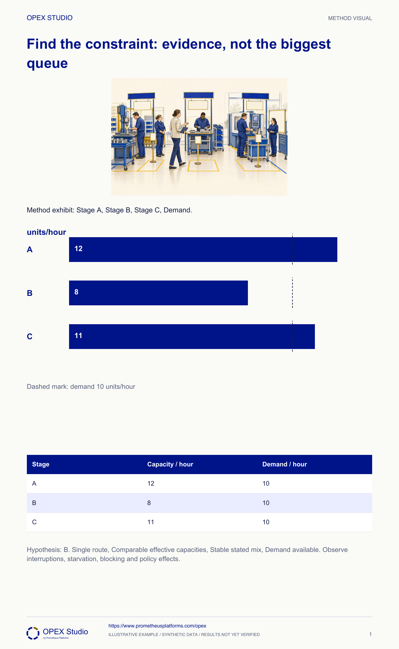
A visible queue is a clue, not a diagnosis. Compare required load with effective capacity over a representative mix and horizon, and observe when processes are starved, blocked or interrupted. In the simple exercise, demand is ten units per hour while stage capacities are twelve, eight and eleven; stage B is the first limiting hypothesis. Real systems need evidence about variability, routing and policies before that conclusion is accepted. The constraint can also be outside the equipment chain, such as demand or an approval rule. Test the hypothesis and recheck it after a material change.

Follow the method

1. Stage A
2. Stage B
3. Stage C
4. Demand

Test the lowest-rate hypothesis against the real route

Fictional three-stage route: A, B and C have supplied comparable effective capacities of 12, 8 and 11 units per hour. Demand is 10 per hour. A snapshot shows the largest visible queue before C, but planner Eli must identify what limits sustained route output under the stated model.

Follow the method

1. Lowest comparable rate
2. Demand relation
3. Largest queue
4. Observed mechanism
5. Improvement claim

The largest queue is a clue, not the conclusion

Use comparable demand and capacity evidence to form a constraint hypothesis, then test it against actual starvation, blocking, quality and release conditions.

Fictional three-stage route: A, B and C have supplied comparable effective capacities of 12, 8 and 11 units per hour. Demand is 10 per hour. A snapshot shows the largest visible queue before C, but planner Eli must identify what limits sustained route output under the stated model.

Role: System analyst working with all three process owners.

Normal condition

The constraint hypothesis explains system delivery within a defined route, mix and period.

The gap

The team assumes the largest current pile must identify the constraint, without checking its release history.

• Single route, comparable effective capacities, stable stated mix and available demand are supplied assumptions.
• The snapshot does not prove steady-state behavior or identify the cause of any capacity loss.

1. Fix the comparison boundary

   Eli confirms that all three capacities refer to the same product route and effective working period. He checks that customer demand is actually available.

   Why: Nameplate rates, different mixes or different calendars cannot be compared as if they represent the same opportunity.

   Evidence: Like-for-like model: 12 / 8 / 11 against demand 10 units/hour.

2. Form the first hypothesis

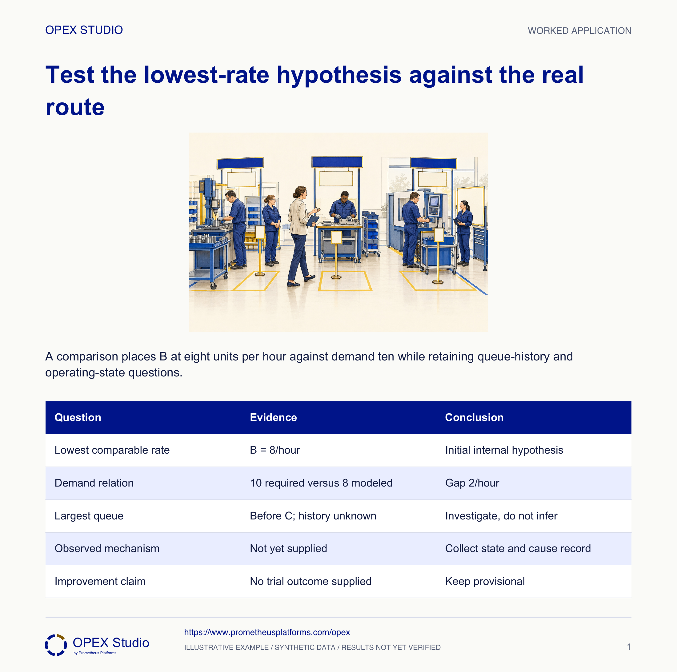
   B at eight units per hour is the lowest supplied rate and below demand. Under the stated assumptions, it is the first internal constraint hypothesis and the modeled gap is two units per hour.

   Why: The arithmetic narrows investigation; it does not by itself establish why B performs at that rate or prove real operating behavior.

   Evidence: Initial model limit 8/hour; demand gap 2/hour.

3. Explain the queue without guessing

   Inspect when the queue before C arrived, whether it contains held or off-route work, and how release batches were scheduled. Record its age and eligibility.

   Why: A queue can reflect earlier releases, quality holds or a temporary event. Its size at one moment does not replace a rate and flow history.

   Evidence: Queue explanation remains open until arrival, status and service history are checked.

4. Observe the candidate’s actual conditions

   Record whether B has ready eligible work, required resources and downstream space. Separate its processing losses from time starved by upstream information or blocked by downstream problems.

   Why: The limiting condition may be a policy, supply or quality issue rather than B’s equipment itself. Improvement must address the actual mechanism.

   Evidence: Observation log distinguishes working, starved, blocked and abnormal states with causes to investigate.

5. Revise the hypothesis when evidence changes

   Compare sustained accepted output and demand after a controlled change. If another condition now limits the system, update the focus and supporting rules.

   Why: A constraint label is not permanent property of a machine. Persisting with an obsolete label is a decision error.

   Evidence: System output, demand basis and current evidence support the next decision.

B is repeatedly starved

Observation shows B often has no ready material because an upstream release rule batches work late, despite A’s average capacity exceeding B’s.

Investigate and test the release/readiness mechanism before assuming more B equipment will solve the loss.

Average capability and timely availability are different. The actual limiting condition may be how work reaches B.

Time-stamped starvation and release evidence guide the revised hypothesis.

Run a practice session

Materials

• Three stage-rate cards, two demand cards and a queue snapshot
• State observation sheet

1. Set the boundary · 4 minutes

   Are these rates genuinely comparable?

2. Choose the first hypothesis · 7 minutes

   Why is the largest queue not enough?

3. Apply the demand-change variant · 9 minutes

   What makes a slow stage become binding?

4. Plan observation · 5 minutes

   Which state would suggest an upstream policy problem?

Debrief

• Challenge unsupported claims from one snapshot.
• Ask learners to name the evidence that would change their mind.

Write assumptions before computing the rate comparison, then choose observations that test the suspected mechanism.

Transfer into the work

Owner: System owner with process and planning representatives

Record: Demand/capacity comparison and time-stamped state observations

Review: After representative observation and every material demand/mix/process change

Evidence: An explanatory hypothesis consistent with accepted delivery and loss states

Revisit the boundary, data comparability or policy mechanism before adding capacity.