Facilitator guide
Case objectives, demonstration plans, debriefs, common mistakes and application checks across all 81 workplace cases and method lessons.
Download Facilitator guide PDF · 166 pages · 65.1 MB OPEXSTUDIO
Verify measurement fitness and process stability.. Follow the visual, practise a decision, then check your thinking.
Fictional teaching examples and AI-generated illustrations. Proposed changes and goals are not achieved results. Use the written instructions and check local conditions before applying a method.
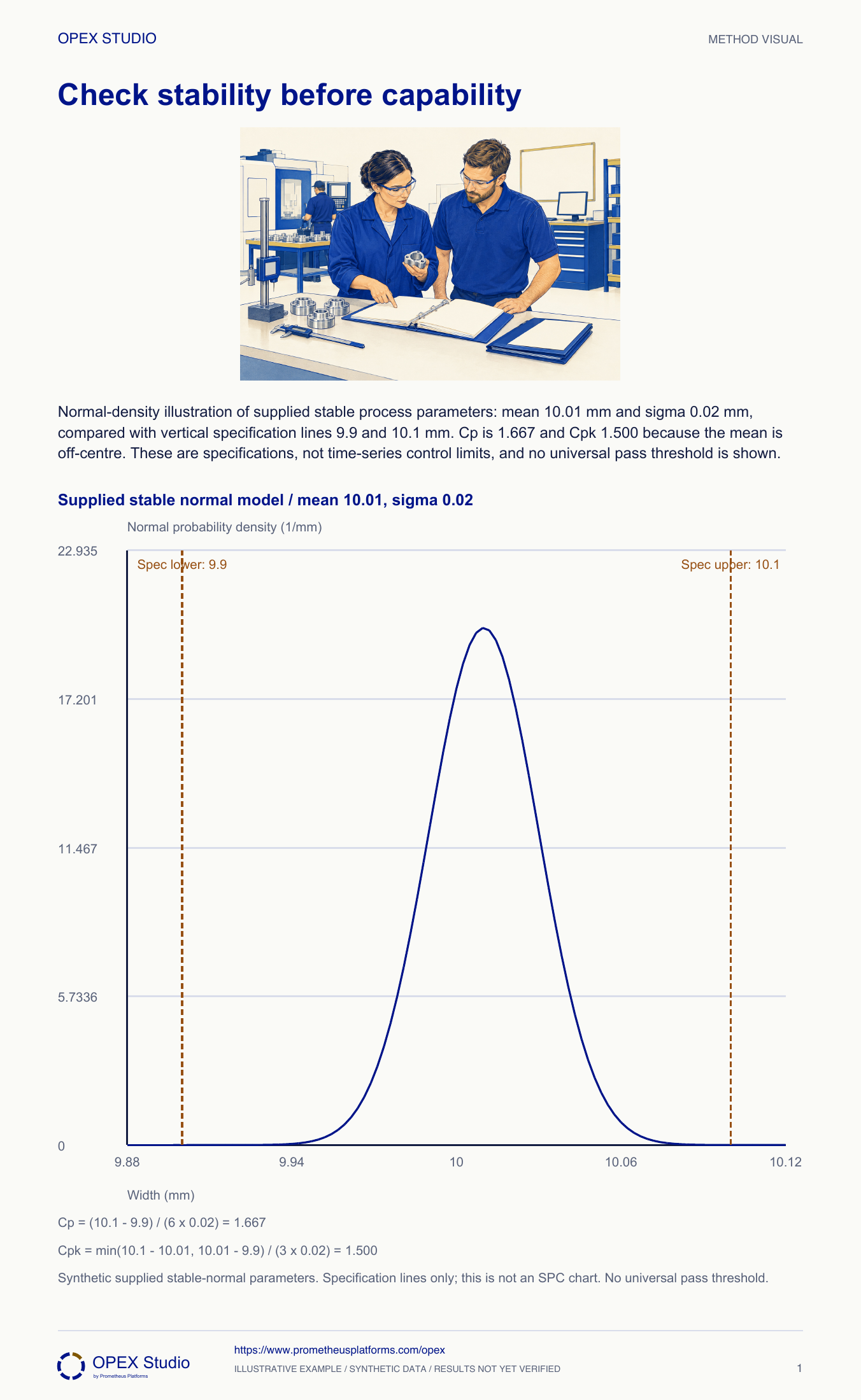
Capability compares a process distribution with stated specification limits. First establish that measurement is fit for the decision and that the process behaviour supports the chosen analysis. Cp compares specification width with six estimated standard deviations; Cpk also reflects how far the mean lies from the nearer specification. An attractive number does not cure instability, establish an applicable customer threshold or remove sampling uncertainty. State the estimator, distribution assumptions and study conditions when reporting results. This example supplies stable-normal parameters solely to demonstrate arithmetic. It is not evidence that a real process is qualified, approved or certain to produce no nonconforming output.
Supplied stable-normal mean10.01,sigma0.02,LSL9.9,USL10.1 mm.
Cp1.667; Cpk1.500; no universal pass threshold implied.
Specification lines describe acceptance requirements, not SPC limits.
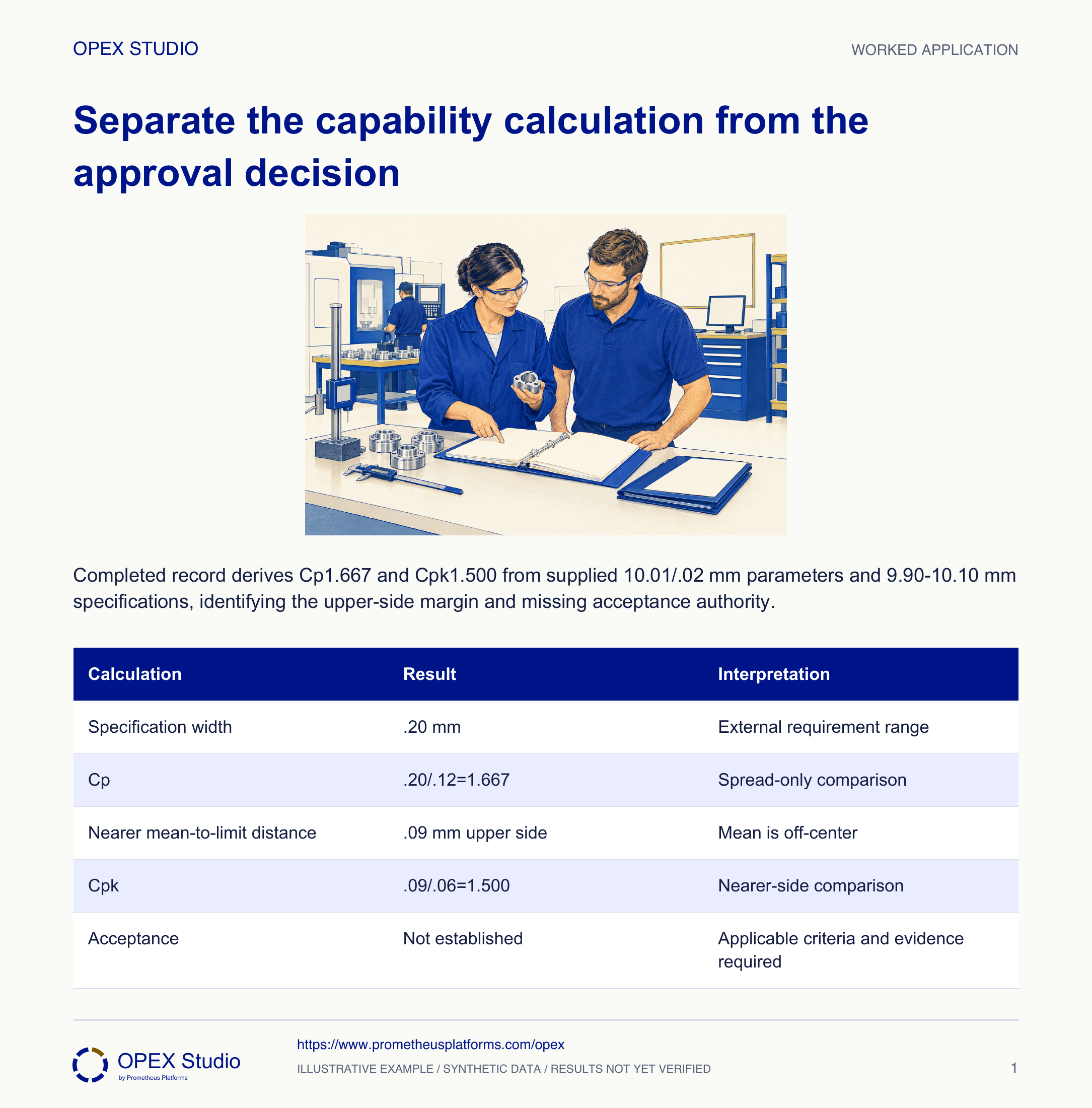
Fictional case: a width process is supplied as stable and approximately normal with mean 10.01 mm and sigma .02 mm. Specifications are 9.90–10.10 mm. These parameters and the existing native distribution remain unchanged. Engineer Asha must explain why Cp and Cpk differ and whether either number authorizes production acceptance.
Cp remains 1.667; Cpk becomes .03/.06=.50. Treat any real drift through process investigation rather than celebrating the unchanged Cp.
The spread-only ratio cannot reveal loss of centering. A changing real process also challenges the stable-distribution premise.
Calculate and interpret Cp and Cpk from explicitly supplied stable-normal parameters while keeping evidence prerequisites and acceptance authority separate.
Fictional case: a width process is supplied as stable and approximately normal with mean 10.01 mm and sigma .02 mm. Specifications are 9.90–10.10 mm. These parameters and the existing native distribution remain unchanged. Engineer Asha must explain why Cp and Cpk differ and whether either number authorizes production acceptance.
Role: Quality engineer with the customer-requirements owner
Distribution, stability, measurement fitness, sampling and specification authority are established for the intended use before a capability conclusion is applied.
A slide presents 1.667 as a universal passing score and treats the six-point SPC illustration from another lesson as proof of this process’s stability.
| Parameter | Supplied value |
|---|---|
| Lower / upper specification | 9.90 /10.10 mm |
| Process mean | 10.01 mm |
| Sigma estimate | .02 mm |
| Assumed model | Stable normal process for this calculation exercise |
| Qualification decision | Not supplied |
Asha identifies specification width 10.10−9.90=.20 mm and records where the actual product requirements would come from. Mean and sigma describe the supplied process, not allowable product limits.
Why: The process distribution and customer tolerance are different authorities. Substituting control limits for specifications would make capability self-referential.
Evidence: The record names LSL, USL, mean and sigma separately.
She labels stable/normal/measurement-suitable as supplied exercise assumptions and lists the actual evidence needed before a real claim. She does not invent a baseline study.
Why: A calculated ratio remains arithmetic even when prerequisites are absent; its predictive capability interpretation would then be unsupported.
Evidence: A prerequisite checklist distinguishes given assumptions from verified workplace records.
Cp=.20/(6×.02)=1.6667, approximately 1.667. This compares specification width with the supplied six-sigma process spread.
Why: Cp alone does not locate the mean within the tolerance. A narrow distribution could still be shifted toward or beyond a specification.
Evidence: The formula retains millimetres in numerator and denominator before cancellation.
Upper distance is 10.10−10.01=.09 mm; lower distance is 10.01−9.90=.11 mm. Cpk=min(.09,.11)/(3×.02)=1.50.
Why: The upper side is closer. The smaller Cpk reflects this off-center mean without changing the supplied spread.
Evidence: The worked record identifies the limiting side and preserves both distances.
Asha reports the two indices under the stated assumptions and requests applicable acceptance requirements and appropriate uncertainty/evidence before a production decision.
Why: Neither number is a universal pass threshold. A capability calculation does not replace process control, customer conditions or the authorized release record.
Evidence: The report states synthetic calculation only and separates interpretation from acceptance.
| Calculation | Result | Interpretation |
|---|---|---|
| Specification width | .20 mm | External requirement range |
| Cp | .20/.12=1.667 | Spread-only comparison |
| Nearer mean-to-limit distance | .09 mm upper side | Mean is off-center |
| Cpk | .09/.06=1.500 | Nearer-side comparison |
| Acceptance | Not established | Applicable criteria and evidence required |
In a hypothetical comparison the mean becomes 10.07 mm while sigma remains .02 mm and specifications stay unchanged.
Cp remains 1.667; Cpk becomes .03/.06=.50. Treat any real drift through process investigation rather than celebrating the unchanged Cp.
The spread-only ratio cannot reveal loss of centering. A changing real process also challenges the stable-distribution premise.
The comparison identifies changed mean, unchanged spread and reduced nearer-side margin.
New synthetic stable-normal parameters are mean 10.02 mm, sigma .025 mm and the same 9.90–10.10 mm specifications.
| Parameter | Value |
|---|---|
| Mean | 10.02 mm |
| Sigma | .025 mm |
| LSL / USL | 9.90 /10.10 mm |
Cp=.20/(6×.025)=1.3333. Cpk=min(.08,.12)/(.075)=1.0667; the upper side limits the result.
These are calculations under supplied assumptions. A real unstable process lacks the fixed-distribution basis of this simple interpretation; acceptance still depends on applicable customer/organizational requirements and suitable evidence.
| Index | Calculation | Rounded result |
|---|---|---|
| Cp | .20/.15 | 1.333 |
| Cpk | .08/.075 | 1.067 |
Which numbers come from requirements and which from the process?
Why is the upper side limiting?
What does the calculation still not prove?
Why can Cp stay constant while risk changes?
Draw the two mean-to-limit distances before calculating Cpk.
Owner: Capability-study owner with customer quality
Record: Study scope, measurement/baseline evidence, indices and applicable decision
Review: Before qualification and after material process changes
Evidence: Traceable data, suitable assumptions and authorized acceptance basis
Resolve instability or measurement gaps before using a capability index as decision evidence.
Capability compares a stable process distribution with specification limits; common indices require explicit distribution and sampling assumptions.
Public primary-source summary; underlying paid standards/forms are not reproduced.Read the lessons online or use these PDFs to prepare, practise and review with your team. No sign-in needed.
Case objectives, demonstration plans, debriefs, common mistakes and application checks across all 81 workplace cases and method lessons.
Download Facilitator guide PDF · 166 pages · 65.1 MBPrintable case worksheets, blank observation records and five calculation exercises; answers are separate.
Download Learner workbook PDF · 169 pages · 10.7 MBReasoned sample responses, worked calculations and coaching guidance; fictional examples are clearly labelled.
Download Answer key and coaching notes PDF · 105 pages · 8.5 MBThe native method mechanisms and worked applications for all 68 detailed lessons, in a separate bookmarked portrait reference.
Download Method and application reference PDF · 141 pages · 10.2 MBFive illustrated system chapters: 15 Flare concept maps and 26 original workplace teaching cards, with links to all 81 supporting cases and method lessons.
Download Illustrated systems atlas PDF · 69 pages · 55.8 MBExplore this connected method and its separate application conditions.
Explore the connected method →Explore this connected method and its separate application conditions.
Explore the connected method →Explore this connected method and its separate application conditions.
Explore the connected method →